Bio-As-2
1. Construct the phylogenetic tree
There are 16 possible changes from one nucleotide to the other. The changes can be represented as 4X4 transition matrix.
| A | C | G | T | |
|---|---|---|---|---|
| A | 0.976 | 0.01 | 0.007 | 0.007 |
| C | 0.002 | 0.983 | 0.005 | 0.01 |
| G | 0.003 | 0.01 | 0.979 | 0.007 |
| T | 0.002 | 0.013 | 0.005 | 0.979 |
Tree Structure-1
Tree Structure-2
Tree Structure-3
python
nucleotide_to_index = {'A': 0, 'C': 1, 'G': 2, 'T': 3}

transition_matrix = np.array([
    [0.976, 0.01, 0.007, 0.007],  # A -> A, C, G, T
    [0.002, 0.983, 0.005, 0.01],   # C -> A, C, G, T
    [0.003, 0.01, 0.979, 0.007],   # G -> A, C, G, T
    [0.002, 0.013, 0.005, 0.979]   # T -> A, C, G, T
])

likelihood = {'A': 0.1, 'C': 0.4, 'G': 0.2, 'T': 0.3}


def F(seq1, seq2):
    likelihood_value = 1
    for i in range(len(seq1)):
        seq1_index = nucleotide_to_index[seq1[i]]
        seq2_index = nucleotide_to_index[seq2[i]]
        transition_prob = transition_matrix[seq1_index, seq2_index]
        # print(transition_prob, likelihood[seq1[i]])
        likelihood_value *= transition_prob * likelihood[seq1[i]]

    return likelihood_value

def calculate_likelihood_For_Tree_1(sequences, hidden_states):
    seq0, seq1, seq2, seq3 = sequences
    likelihood_value = 0
    for hidden in hidden_states:
        likelihood_value += (F(seq0, hidden) * F(seq0, seq3) * F(hidden, seq1) * F(hidden, seq2))
    return likelihood_value


def calculate_likelihood_For_Tree_2(sequences, hidden_states):
    seq0, seq1, seq2, seq3 = sequences
    likelihood_value = 0
    for hidden in hidden_states:
        likelihood_value += (F(seq0, seq1) * F(seq0, seq3) * F(hidden, seq1) * F(hidden, seq2))
    return likelihood_value

def calculate_likelihood_For_Tree_3(sequences, hidden_states):
    seq0, seq1, seq2, seq3 = sequences
    likelihood_value = 0
    for hidden in hidden_states:
        likelihood_value += (F(seq0, seq2) * F(seq0, hidden) * F(hidden, seq1) * F(hidden, seq3))
    return likelihood_value


sequences = ["AGA", "AGC", "ACT", "ACG"]

def generate_hidden_states():
    return [''.join(state) for state in product(nucleotide_to_index.keys(), repeat=3)]

hidden_states = generate_hidden_states()
likelihood_value_1 = calculate_likelihood_For_Tree_1(sequences, hidden_states)
likelihood_value_2 = calculate_likelihood_For_Tree_2(sequences, hidden_states)
likelihood_value_3 = calculate_likelihood_For_Tree_3(sequences, hidden_states)
print(f"Tree Structure 1: {likelihood_value_1}")
print(f"Tree Structure 2: {likelihood_value_2}")
print(f"Tree Structure 3: {likelihood_value_3}")
2. Please download the gene expression table from iSpace. Refers to lab 2 and lab 3,
1. Apply cell type cluster for the data. (Please store the cluster label for each cell);
python
from sklearn.cluster import AgglomerativeClustering

model=AgglomerativeClustering(n_clusters=10,metric='euclidean',linkage='ward')

cluster_labels = model.fit_predict(data_umap)
2. For the two clusters that have most cells (summary the numbers as table), detect the differential expressed genes across the two cluster. Remember to conduct multiple test adjustment. (Please store pvalue, and fold change for each gene; Alpha=0.05, fold change >2 as threshold)
python
from scipy.stats import ttest_ind
import numpy as np
import pandas as pd
# 初始化存储结果的列表
genes = filtered_data.columns
pvalues = []
fold_changes = []
# 对每个基因计算 P 值和 Fold Change
for gene in genes:
group1 = cluster_1_data[gene]
group2 = cluster_2_data[gene]
# T 检验
t_stat, p_value = ttest_ind(group1, group2, equal_var=False)
pvalues.append(p_value)
# Fold Change
mean_group1 = np.mean(group1)
mean_group2 = np.mean(group2)
fold_change = mean_group1 / mean_group2 if mean_group2 != 0 else np.inf
fold_changes.append(fold_change)
# 创建结果 DataFrame
diff_genes = pd.DataFrame({
'Gene': genes,
'PValue': pvalues,
'FoldChange': fold_changes
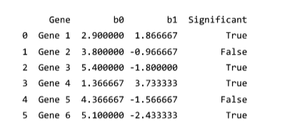
})3. For the detected differential expressed genes, apply the gene set enrichment to see what is the most relative biological function.
python
from gprofiler import GProfiler

# 初始化 GProfiler 实例
gp = GProfiler(return_dataframe=True)

# 获取显著差异表达基因的列表
significant_genes_list = significant_genes['Gene'].tolist()

# 运行基因集富集分析
enrichment_results = gp.profile(
    organism='hsapiens',  # 人类
    query=significant_genes_list  # 差异表达基因
)

# 保存结果
enrichment_results.to_csv('gene_enrichment_results.csv', index=False)

# 打印前几行结果
print(enrichment_results.head())
print("基因集富集分析完成,结果已保存到 gene_enrichment_results.csv")
3.
4. Network reconstruction. Given gene expression table as follow,
Please calculate the mutual information between each gene pair (see mutinformation() in R package “infotheo").
Apply CLR (Context Likelihood of Relatedness) for each pair.
Plot the inferred network with CLR=0.1 as threshold.
python
import pandas as pd
from sklearn.metrics import mutual_info_score
import numpy as np
import networkx as nx
import matplotlib.pyplot as plt


data = {
    "G1": [5, 4, 4, 5, 3, 6],
    "G2": [2, 3, 3, 7, 2, 5],
    "G3": [3, 2, 3, 4, 3, 6],
    "G4": [3, 3, 3, 6, 1, 3]
}
df = pd.DataFrame(data)


genes = df.columns
n_genes = len(genes)
mi_matrix = np.zeros((n_genes, n_genes))

for i in range(n_genes):
    for j in range(n_genes):
        if i != j:
            mi_matrix[i, j] = mutual_info_score(df[genes[i]], df[genes[j]])


clr_matrix = np.zeros_like(mi_matrix)
for i in range(n_genes):
    for j in range(n_genes):
        if i != j:
            z_i = (mi_matrix[i, j] - np.mean(mi_matrix[i, :])) / np.std(mi_matrix[i, :])
            z_j = (mi_matrix[i, j] - np.mean(mi_matrix[:, j])) / np.std(mi_matrix[:, j])
            clr_matrix[i, j] = np.sqrt(z_i**2 + z_j**2)


threshold = 0.1
edges = []
for i in range(n_genes):
    for j in range(i + 1, n_genes):
        if clr_matrix[i, j] > threshold:
            edges.append((genes[i], genes[j], clr_matrix[i, j]))


G = nx.Graph()
for edge in edges:
    G.add_edge(edge[0], edge[1], weight=edge[2])

pos = nx.spring_layout(G)
nx.draw(G, pos, with_labels=True, node_color='lightblue', node_size=2000, font_size=12)
nx.draw_networkx_edge_labels(G, pos, edge_labels={(u, v): f"{d['weight']:.2f}" for u, v, d in G.edges(data=True)})
plt.title('Inferred Gene Network (CLR > 0.1)')
plt.show()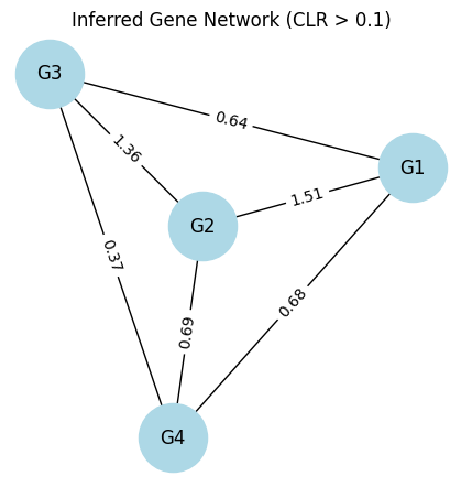
5. Open Question
To infer which cancer type a patient might have based on their mutation signature, follow these steps:
- Collect Mutation Data: For each patient, obtain their mutation counts across the different mutation types.
- Construct a Mutation Vector: Create a 1x96 vector representing the counts of each mutation type.
- Compare with Signatures: Use the mutation signatures obtained from NMF. Calculate the similarity/distance between the patient's vector and each signature.
- Identify Closest Signature: Determine the signature that best matches the patient's mutation vector.
- Map to Cancer Types: Use the contribution matrix (H) from the NMF to identify the associated cancer types for the closest signature.
By following these steps, you can infer the likely cancer type for the patient based on their mutation profile.