10-CG-Rasterization
Overview of Rasterization
Framebuffer Model
- Raster Display: 2D array of picture elements (pixels)
- Pixels individually set/cleared (greyscale, color)
- Window coordinates: pixels centered at integers
2D Scan Conversion
Geometric primitives
- (point, line, polygon, circle, polyhedron, sphere... )
Primitives are continuous; screen is discrete
Scan Conversion:
- algorithms for efficient generation of the samples comprising this approximation
将连续的几何图元(如点、直线、多边形、圆等)转换为离散像素集合的过程,称为扫描转换(Scan Conversion)。其核心是通过算法高效地确定图元覆盖的像素,并设置相应的颜色值。
核心问题:
- 几何图元是数学上的连续对象(如直线是无限个点的集合),而屏幕是离散的像素阵列,需用有限像素近似表示图元。
- 目标:找到最接近图元的像素集合,同时保证效率(如减少浮点运算、避免冗余判断)。
典型图元的扫描转换:
点(Point):
- 直接将坐标
对应的像素设置为指定颜色。 - 若坐标为非整数,需通过插值(如四舍五入)确定像素中心。
- 直接将坐标
直线(Line):
- 问题:给定两点
和 ,确定覆盖的像素。 - 算法:
- Bresenham算法:仅用整数运算,通过误差累积确定下一个像素,效率极高。
- 中点画线法:利用中点误差判断像素位置,适用于硬件实现。
- 示例: 绘制从
到 的直线,覆盖像素为 、 、 、 。
- 问题:给定两点
多边形(Polygon):
- 问题:填充多边形内部区域对应的像素。
- 算法:
- 扫描线算法:按行(扫描线)遍历多边形,确定每行的像素区间,填充区间内的像素。
- **奇偶规则(Odd-Even Rule)或非零环绕数规则(Non-Zero Winding Number Rule)**判断点是否在多边形内部。
- 示例: 左图为连续多边形,右图为扫描转换后的像素填充结果(绿色和蓝色像素)。
圆(Circle):
- 算法:中点画圆法、Bresenham画圆法,利用对称性减少计算量(仅计算1/8圆,镜像生成其余部分)。
Brute force solution for triangles
For each pixel
- Compute line equations at pixel center
- "clip" against the triangle
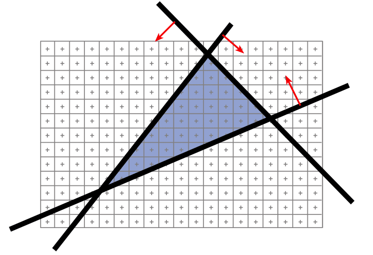
Improvement:
- Compute only for the screen bounding box of the triangle
- Xmin, Xmax, Ymin, Ymax of the triangle vertices
Better Solution: Line rasterization
Line Rasterization Requirements
- Transform continuous primitive into discrete samples
- Uniform thickness & brightness
- Continuous appearance
- No gaps
- Accuracy
- Speed
Algorithm Design Choices
Assume
Exactly one pixel per column
- Avoid
,
亮度变化、最大差异与抗锯齿补偿
亮度随斜率变化的原因:像素密度差异
现象描述: 当直线斜率不同时,光栅化后的像素密度不同,导致视觉亮度差异。
- 水平线段(
):像素沿x轴密集排列,单位长度内像素数最多,亮度最高; - 对角线段(
):像素沿x、y轴交替排列,单位长度内像素数最少,亮度最低。
数学分析:
假设线段长度为
,水平线段的像素数约为 (dx = L),对角线段的像素数约为 (dx = dy = L / )。 亮度与像素数成正比,因此对角线段的亮度约为水平线段的
,即亮度差异最大可达 倍(水平线段亮度是对角线段的 倍)。 Compensate for this
- 抗锯齿技术: 通过调整像素亮度权重,补偿因像素离散化导致的亮度不均和锯齿,使不同斜率的线段视觉效果更一致。
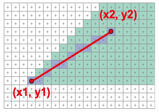
Line Rasterization
Naive Line Rasterization Algorithm
- Simply compute
as a function of - Conceptually: move vertical scan line from
to - Set pixel
- Conceptually: move vertical scan line from
Code
void Line (int x,, int yi, int x2, int y){
int x;
float dy, dx, y, m;
dy = y2 - y1;
dx = x2 - X1;
m = dy/dx;
y= y1;
for (x = x1; x<=x2, X++) {
WritePixel (x, round (y)) ;
y += m;
}
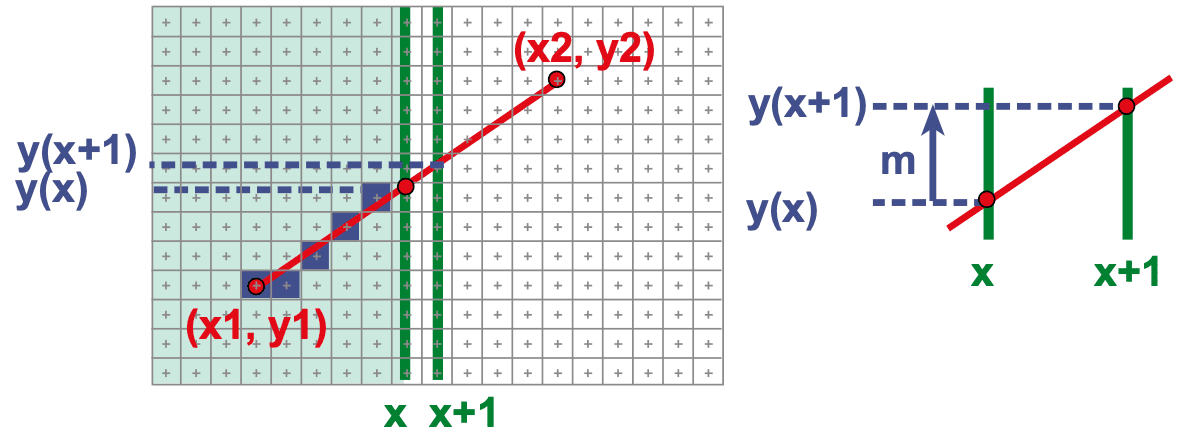
}Efficiency
- Computing
value is expensive - Observe:
at each step
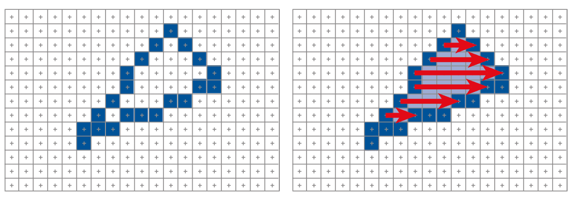
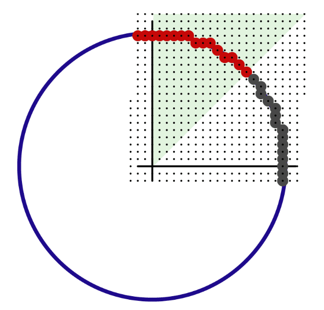
Grid Marching vs. Line Rasterization
网格行进 vs. 直线光栅化:目标驱动的方法差异** 图示对比解析:
左图:光线加速(Ray Acceleration)
- 场景:光线穿过网格,需检测所有与之相交的单元格(如红色网格)。
- 目的:在光线追踪中加速交点计算,减少不必要的物体检测。
- 特点:遍历所有穿过的单元格,计算量大,但确保无遗漏。
中图与右图:直线光栅化
- 场景:在像素网格中找到最接近直线的像素(如红色像素)。
- 目的:用离散像素近似连续直线,需平衡精度与效率。
- 特点:
- 中图(灰色像素):可能包含边缘模糊的抗锯齿处理;
- 右图:纯二值化像素,严格选择最近点。
关键区别:
| 维度 | 网格行进(光线追踪) | 直线光栅化 |
|---|---|---|
| 核心任务 | 几何相交检测 | 离散化采样(像素选择) |
| 输出粒度 | 网格单元格(可能多个) | 像素点(单个或加权像素) |
| 计算重点 | 射线方向与网格交点 | 像素与直线的距离或误差 |
| 算法目标 | 无遗漏地检测所有可能相交的物体 | 用最少计算量生成视觉连贯的线段 |
- Ray Acceleration: Must examine every cell the line touches
- Line Rasterization: Best discrete approximation of the line
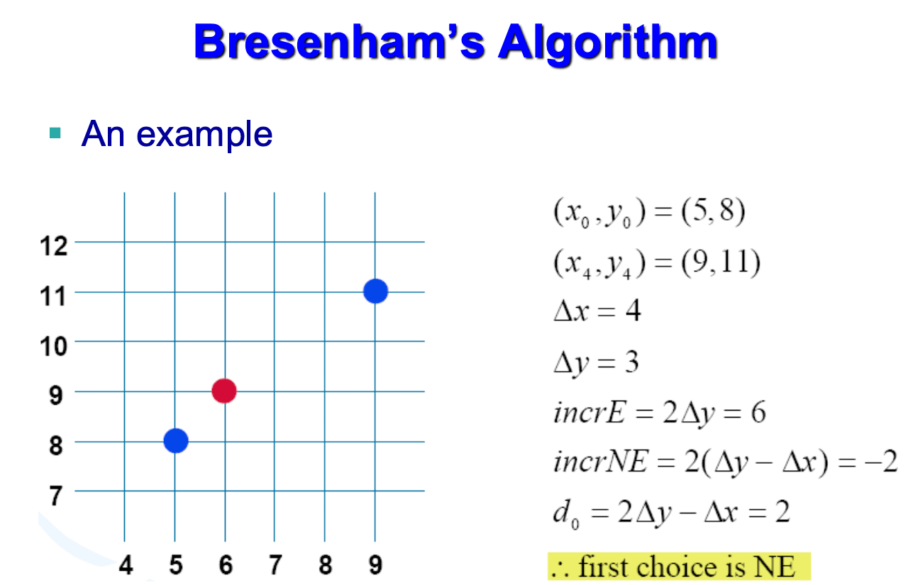
Bresenham's Algorithm (DDA)
- Digital differential analyzer(DDA)
Select pixel vertically closest to line segment
- intuitive, efficient,
- pixel center always within 0.5 vertically
Observation:
- If we're at pixel
, the next pixel must be either or 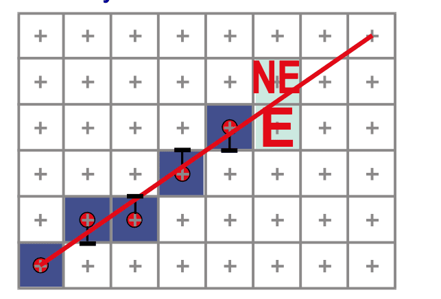
Which pixel to choose: E or NE?
- Choose E if segment passes below or through middle point M
- Choose NE if segment passes above M
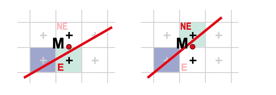
Use decision function F to identify points underlying line L:
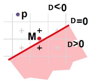
- positive below L
- zero on L
- negative above L
- If
, M lies above the line, chose E - If
, M lies below the line, chose NE
中点M的坐标: E和NE像素的中点为
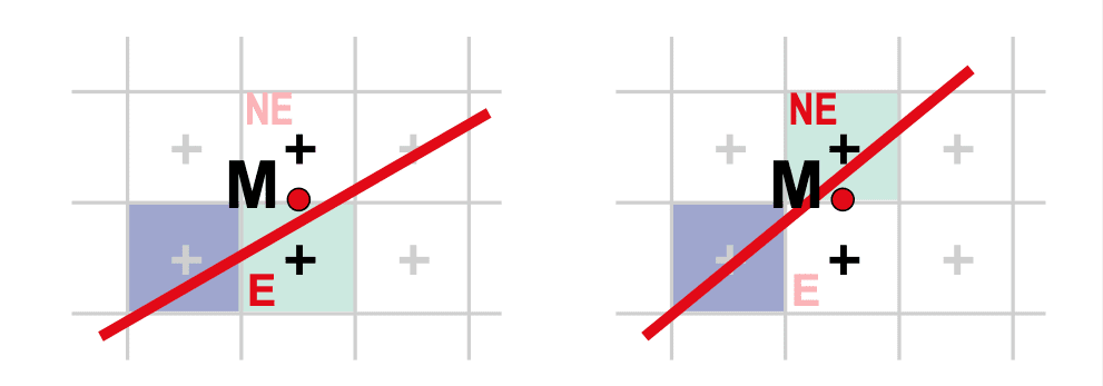
关键问题:
包含浮点数 ,需整数化处理以避免浮点运算。 - 决策仅需
的符号(正/负),因此可将其乘以2(符号不变): 此时 为整数,且: → 在直线上方 → 选 ; → 在直线下方 → 选 ; → 直线经过 ,约定选 。
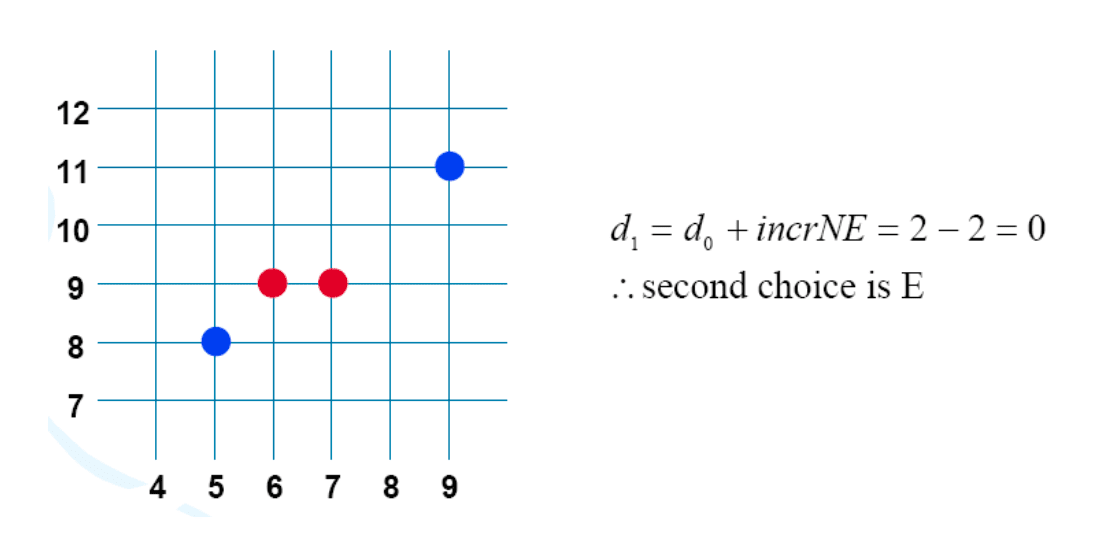
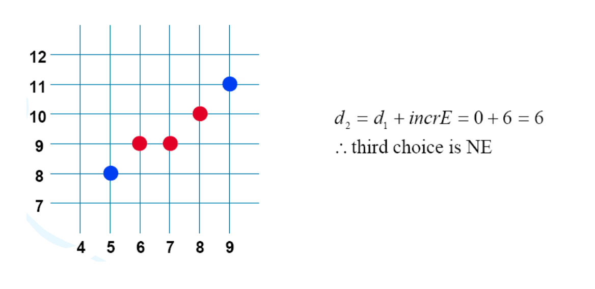
决策函数的递推优化:增量计算避免重复运算目标:避免每次计算
推导过程:
展开
: 注意到
(因 在直线上),故: 代入
得: 递推关系:
- 若选
( 不变): 下一个中点为 ,代入 得: - 若选
( 递增1): 下一个中点为 ,代入 得:
- 若选
起点
这是递推计算的起点,无需额外计算。
void BresenhamLine(int x0, int y0, int xn, int yn) {
    int dx, dy, incrE, incrNE, d, x, y;
    dx = xn - x0;       // x方向总增量(假设xn > x0)
    dy = yn - y0;       // y方向总增量(正斜率时dy > 0)
    d = 2*dy - dx;      // 初始决策变量d0 = 2Δy - Δx
    incrE = 2*dy;       // 选择E像素时d的增量(2Δy)
    incrNE = 2*dy - 2*dx; // 选择NE像素时d的增量(2Δy - 2Δx)
    x = x0; y = y0;     // 初始化当前像素为起点
    DrawPixel(x, y);    // 绘制起点
    while (x < xn) {    // 逐列扫描,x从起点到终点
        if (d <= 0) {   // 若d≤0,直线在中点M下方或经过M,选E像素
            d += incrE; // d更新为d + 2Δy
            x++;        // 右移一列(y不变)
        } else {        // 若d>0,直线在中点M上方,选NE像素
            d += incrNE; // d更新为d + 2Δy - 2Δx
            x++; y++;   // 右移一列且上移一行
        }
        DrawPixel(x, y); // 绘制当前像素
    }
}
Example
Filling Polygons
Scan Line Algorithm
- Compute the bounding pixels
- Fill the span
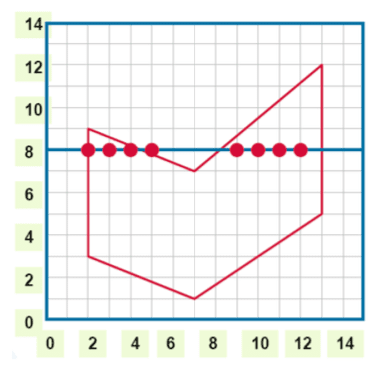
- Find the intersections of current scan line with all edges of the polygon.
- Sort the intersections by increasing x coordinate.
- Fill in pixels that lie between pairs of intersections that lie interior to the polygon using the odd/even parity rule.
- Parity: even, change parity once encounter an edge
- Special parity: no change of the parity (draw 1 pixel)
Construction Edge Table
Circle Rasterization
Generate pixels for 2nd octant only
slope progress from
Analog of Bresenham Segment Algorithm
Decision Function
, point in the circle , point on the circle , point not in the circle
Initialize:
error term
On each iteration: update x:
误差项设计
为避免浮点运算,引入误差项
:点在圆内(因 ); :点在圆上; :点在圆外(因 )。
目标:通过比较
算法步进逻辑:从
初始点:圆心为
每步操作:
- x递增1:
(因在第二八分圆,x方向单增)。 - 更新误差项:
- 判断是否需要调整y:
- 若
:点仍在圆内,y不变,选右侧像素E ; - 若
:点接近圆外,y递减1,选右下像素SE ,并修正误差项:$$e' = e' + (2y - 1).$$ 因 增量为 ,即误差项增量为
- 若
void CircleRasterization(int xc, int yc, int R) {
    int x = 0, y = R;
    float e = 0; // 误差项初始化为0
    DrawOctants(xc, yc, x, y); // 绘制八对称像素

    while (x < y) {
        x++;
        e -= 2 * x + 1; // 更新误差项(x递增1)
        if (e < 0.5) { // 需调整y
            y--;
            e += 2 * y - 1; // y递减1,更新误差项
        }
        DrawOctants(xc, yc, x, y); // 绘制当前像素的八对称点
    }
}

void DrawOctants(int xc, int yc, int x, int y) {
    // 绘制八对称的8个像素
    SetPixel(xc + x, yc + y);
    SetPixel(xc + y, yc + x);
    SetPixel(xc + y, yc - x);
    SetPixel(xc + x, yc - y);
    SetPixel(xc - x, yc - y);
    SetPixel(xc - y, yc - x);
    SetPixel(xc - y, yc + x);
    SetPixel(xc - x, yc + y);
}