07-CG-Curves

---

Bezier Curve

Linear Bezier curve ($n=1$):

$$F(u)=P_0(1-u)+P_{1}u$$

which represents a straight - line segment between two control points $P_0$ and $P_1$.

Quadratic Bezier curve ($n=2$): $$F(u)=P_{0}(1 - u)^{2}+P_{1}[2u(1 - u)]+P_{2}u^{2}$$ determined by three control points $P_0$, $P_1$, and $P_2$. It can form a simple curved shape.

Cubic Bezier curve ($n=3$):

$$F(u)=P_0(1-u{)}^3+P_1[3u(1-u{)}^2]+P_2[3u^2(1-u)]+P_3{u}^3$$

with four control points $P_0$, $P_1$, $P_2$, and $P_3$. Cubic Bezier curves are very common in graphics and can create a wide variety of complex curves.

$$F(u)=P_0(1-u{)}^3+P_1[3u(1-u{)}^2]+P_2[3u^2(1-u)]+P_3{u}^3$$$$=(u^3{u}^{2}u1)\left(\begin{array}{cccc}-1& 3& -3& 1\\ 3& -6& 3& 0\\ -3& 3& 0& 0\\ 1& 0& 0& 0\end{array}\right)\left(\begin{array}{c}{P}_0\\ P_1\\ P_2\\ P_3\end{array}\right)$$

Power basis: $[u^3{u}^{2}u1]$Spline basis:

$$\left(\begin{array}{cccc}-1& 3& -3& 1\\ 3& -6& 3& 0\\ -3& 3& 0& 0\\ 1& 0& 0& 0\end{array}\right)$$

Geometry: $[P_0{P}_1{P}_2{P}_3{]}^T$

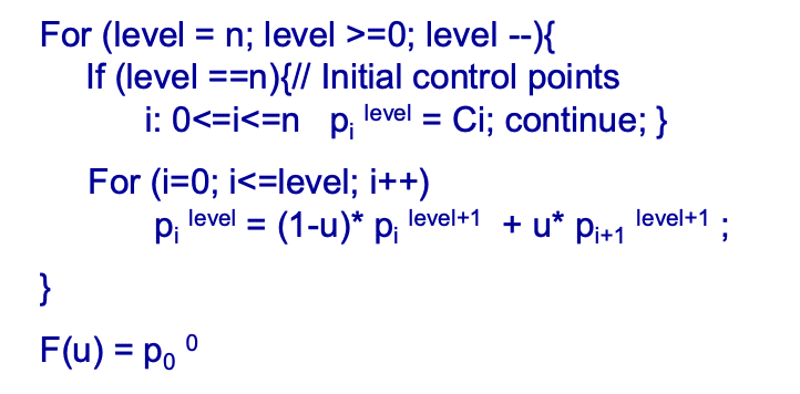
DeCasteljau Implementation

• Input: Control points Ci with 0<=i<=n where n is the degree.
• Output: F(u) where u is the parameter for evaluation

def decasteljau(control_points, u):
    """
    Evaluate a point on a Bézier curve using the DeCasteljau algorithm.
    
    Parameters:
    control_points (list of tuples): List of control points (x, y) for the curve.
    u (float): Parameter value in [0, 1] to evaluate the curve at.
    
    Returns:
    tuple: The resulting point (x, y) on the Bézier curve.
    """
    n = len(control_points) - 1  # Degree of the curve (n = len(control_points) - 1)
    points = [list(point) for point in control_points]  # Convert to mutable lists
    
    # Iterate from the highest level down to level 0
    for level in range(n, 0, -1):  # Levels: n, n-1, ..., 1
        for i in range(level):
            # Linearly interpolate between consecutive points at the current level
            x = (1 - u) * points[i][0] + u * points[i + 1][0]
            y = (1 - u) * points[i][1] + u * points[i + 1][1]
            points[i] = [x, y]  # Update the point for the next level
    
    return tuple(points[0])  # Return the final point as a tuple

Bernstein-Bezier polynomial basis

• Linear combination of basis functions: Bezier curves are expressed as a linear combination of Bernstein
• Bezier polynomials. For a curve of degree $n$, it is given by$$F(u)=\sum _{k=0}^n{P}_k{B}_k^n(u)$$
• where $P_k$ are the control points that influence the shape of the curve, $u\in [0,1]$ is the parameter, and $$B_{k}^{n}(u)=\frac{n!}{k!(n - k)!}(1 - u)^{n - k}u^{k}$$ are the Bernstein - Bezier polynomials.

Key Properties

Interpolation at end-points, but approximation at other points

• Global Influence: Single piece, moving one point affects whole curve (no local control as in B-splines later)
• Geometric Invariance: Invariant to translations, rotations, scales etc.That is, translating all control points translates entire curve.
• Ease of Subdivision: Easily subdivided into parts for drawing: Hence, Bezier curves easiest for drawing

Interpolation Curve – over constrained cause lots of (undesirable) oscillations

Approximation Curve – more reasonable

Polar form labeling (blossoms)

Labeling trick for control points and intermediate deCasteljau points that makes thing intuitive

Why Polar Forms:

• Simple mnemonic: which points to interpolate and how in deCasteljau algorithm
• Easy to see how to subdivide Bezier curve which is useful for drawing recursively
• Generalizes to arbitrary spline curves

Termination Criteria

a. Geometric Tolerance (Most Common)

• Criterion: The distance between the start and end points of the curve segment is smaller than a predefined tolerance (ε).
  • Rationale: When the curve segment is sufficiently "straight" (or close to a line), it can be approximated by a straight line segment for rendering.

b. Recursion Depth Limit

• Criterion: The number of recursive subdivisions exceeds a maximum allowed depth (e.g., max_depth).
  • Rationale: Prevents infinite recursion due to numerical errors or pathological cases (e.g., curves that never flatten sufficiently).

c. Screen Space Error

• Criterion: The projected length of the curve segment on the screen is smaller than a single pixel.
  • Rationale: Used in computer graphics to match the display resolution (e.g., 1 pixel error is visually imperceptible).

Pseudo Code for Recursive Subdivision Rendering

Below is a generic pseudo code for rendering a Bezier curve via recursive subdivision, using geometric tolerance as the termination criterion.

RENDER_BEZIER(control_points, tolerance, current_depth, max_depth):
    if NUMBER_OF_CONTROL_POINTS(control_points) == 2:
        // Base case: line segment, draw directly
        DRAW_LINE(control_points[0], control_points[1])
        return
  
    // Check termination criteria
    if DISTANCE(control_points[0], control_points[-1]) < tolerance OR current_depth > max_depth:
        // Approximate with a line segment
        DRAW_LINE(control_points[0], control_points[-1])
        return
  
    // Subdivide the curve using de Casteljau algorithm
    u = 0.5  // Subdivide at the midpoint (common choice, but u can be any parameter)
    left_control_points, right_control_points = DECASTELJAU_SUBDIVIDE(control_points, u)
  
    // Recurse on left and right segments
    RENDER_BEZIER(left_control_points, tolerance, current_depth + 1, max_depth)
    RENDER_BEZIER(right_control_points, tolerance, current_depth + 1, max_depth)

Bezier:Disadvantages

• Single piece, no local control
• Complex shapes: can be very high degree, difficult
• Continuity defects during segmented splicing

Continuity definitions

• $C^0$ continuous

  • Curve/surface has no breaks, gaps, or holes.

• $G^1$ continuous

  • Tangent at joint has the same direction.

• $C^1$ continuous

  • Curve/surface derivative is continuous.
  • Tangent at joint has the same direction and magnitude.

• $C^n$ continuous

  • Curve/surface through $n^{\text{th}}$ derivative is continuous.
  • Important for shading.

Relationship Between the # of control points, and the # of cubic Bézier subcurves:

Let:

• $n$ = number of cubic Bézier subcurves,
• $N$ = total number of control points.

Formula:

$$N=3n+1$$

B-spline curves

• Cubic B-splines have $C^2$ continuity, local control
• Curve is not constrained to pass through any control points
• 4 segments per control point, 4 control points per segment
• Knots where two segments join: Knotvector
• Knotvector uniform/non-uniform (we only consider uniform cubic B-splines, not general NURBS)
  • BSpline: uniform cubic BSpline
  • NURBS: Non-Uniform Rational BSpline
    • non-uniform = different spacing between the blending functions, a.k.a. knots
    • rational = ratio of polynomials (instead of cubic)

Polar Forms: Cubic Bspline Curve

• Labeling little different from in Bezier curve
• No interpolation of end-points like in Bezier
• Advantage of polar forms: easy to generalize