Bayesian Network Parameter Learning

The Maximum Likelihood Estimation (MLE)

Bayesian Maximum A Posterior (MAP)

1. $\theta$ is a continuous random variable that takes values in $[0,1]$.

2. Assumption: prior probability distribution of $\theta$: $p(\theta )$.
   It is our beliefs about the parameter before seeing the data.

3. [Output] The posterior probability distribution of $\theta$:

   $$p(\theta \mid D)$$

   It is the updated distribution of the parameter after seeing the data.
   It gives us an estimate, i.e., the mean of the distribution, but also measures uncertainty about the estimate, i.e., standard deviation.

4. Prediction of $D_{n+1}$ using the i.i.d. property:

   $$P(D_{n+1}=H\mid D)=\int P(D_{n+1}=H\mid \theta ,D)p(\theta \mid D)d\theta$$$$=\int P(D_{n+1}=H\mid \theta )p(\theta \mid D)d\theta$$$$=\int \theta p(\theta \mid D)d\theta$$

   Full Bayesian: Take expectation over $\theta$ through the integral.

5. The computation of the integral of the full Bayesian estimate can be complicated.
   We can use $maxp(\theta \mid D)$ instead.

6. Bayesian methods involve a degree of subjectivity, as the choice of the prior can influence the results (posterior), especially when the data is sparse or the model is complex, while MLE does not.

$$P(D_{n+1}=H\mid D)={\theta }_{\text{MAP}}=\arg maxp(\theta \mid D)$$

The value of the parameter that maximizes the posterior distribution.

Recall Bayes' Theorem:

$$P(\theta \mid D)=\frac{P(D\mid \theta )p(\theta )}{P(D)}$$

Where $P(D\mid \theta )$ is the likelihood $L(\theta \mid D)$ of the observed data $D$, and $P(D)$ does not depend on $\theta$, acting as a constant.

---

整个推导分为三个阶段：

1. 准备阶段：定义似然函数和先验分布。
2. 更新阶段：利用贝叶斯定理计算后验分布。
3. 预测阶段：通过全贝叶斯积分得出最终公式。

---

第一阶段：准备原材料

我们需要两个核心组件：

1. 似然函数 (Likelihood) $P(D\mid \theta$) 这是描述数据如何产生的。假设掷硬币服从二项分布，参数 $\theta$ 代表正面概率。

$$P(D|\theta )={\theta }^{n_H}(1-\theta {)}^{n_T}$$

2. 先验分布 (Prior) $p$(\theta$) 我们选择 Beta 分布 作为先验，因为它和二项分布是“共轭”的（数学形式相似，好计算）。

$$p(\theta )=\frac{\mathrm{\Gamma }(\alpha )}{\mathrm{\Gamma }({\alpha }_H)\mathrm{\Gamma }({\alpha }_T)}{\theta }^{{\alpha }_H-1}(1-\theta {)}^{{\alpha }_T-1}$$

• 为了书写方便，我们把前面的 Gamma 函数系数统称为常数 $C_{prior}$。
• ${\alpha }_H,{\alpha }_T$ 是先验的超参数（虚拟计数）。

---

第二阶段：计算后验分布 (Posterior)

根据贝叶斯定理：

$$p(\theta |D)=\frac{P(D|\theta )p(\theta )}{P(D)}\propto P(D|\theta )p(\theta )$$

由于分母 $P(D)$ 与 $\theta$ 无关，我们可以先忽略常数，只看与 $\theta$ 有关的核心部分 。

步骤：

1. 将似然和先验相乘：

$$p(\theta |D)\propto [{\theta }^{n_H}(1-\theta {)}^{n_T}]\cdot [{\theta }^{{\alpha }_H-1}(1-\theta {)}^{{\alpha }_T-1}]$$

2. 合并同类项（指数相加）：

$$p(\theta |D)\propto {\theta }^{(n_H+{\alpha }_H)-1}(1-\theta {)}^{(n_T+{\alpha }_T)-1}$$

结论： 观察这个式子，它的形式依然是一个 Beta 分布！ 新的参数变成了：

• 新正面计数：${\alpha }_H^{\prime }={\alpha }_H+n_H$
• 新反面计数：${\alpha }_T^{\prime }={\alpha }_T+n_T$

所以，后验分布的完整概率密度函数（加上归一化常数）是：

$$p(\theta |D)=\underset{\text{新的归一化常数 }{C}_{new}}{\underbrace{\frac{\mathrm{\Gamma }(n+\alpha )}{\mathrm{\Gamma }(n_H+{\alpha }_H)\mathrm{\Gamma }(n_T+{\alpha }_T)}}}\cdot {\theta }^{n_H+{\alpha }_H-1}(1-\theta {)}^{n_T+{\alpha }_T-1}$$

(注：这里 n=nH​+nT​ 是总数据量，α=αH​+αT​ 是总先验量)

---

第三阶段：全贝叶斯预测 (Prediction)

这是最关键的一步。我们要预测下一次是正面，不是只取一个 $\theta$，而是对所有可能的 $\theta$ 求加权平均（积分）。

目标公式：

$$P(D_{n+1}=H|D)={\int }_0^{1}P(D_{n+1}=H|\theta )\cdot p(\theta |D)d\theta$$

因为 $P(D_{n+1}=H|\theta )=\theta$，所以变成：

$$={\int }_0^1\theta \cdot p(\theta |D)d\theta$$

推导步骤：

1. 代入后验分布：

$$={\int }_0^1\theta \cdot [C_{new}\cdot {\theta }^{n_H+{\alpha }_H-1}(1-\theta {)}^{n_T+{\alpha }_T-1}]d\theta$$

2. 合并 $\theta$： 积分里的 $\theta$ 和后面的 ${\theta }^{...-1}$ 合并，$-1$ 消失了：

$$=C_{new}{\int }_0^1{\theta }^{n_H+{\alpha }_H}(1-\theta {)}^{n_T+{\alpha }_T-1}d\theta$$

3. 利用 Beta 函数的定义求解积分： 数学上已知：${\int }_0^1{x}^{a-1}(1-x{)}^{b-1}dx=\frac{\mathrm{\Gamma }(a)\mathrm{\Gamma }(b)}{\mathrm{\Gamma }(a+b)}$。 对比我们的积分项：

   • 指数 $n_H+{\alpha }_H$ 对应公式里的 $a-1⟹a=n_H+{\alpha }_H+1$
   • 指数 $n_T+{\alpha }_T-1$ 对应公式里的 $b-1⟹b=n_T+{\alpha }_T$

所以，积分部分的结果是：

$$\frac{\mathrm{\Gamma }(n_H+{\alpha }_H+1)\mathrm{\Gamma }(n_T+{\alpha }_T)}{\mathrm{\Gamma }(n_H+{\alpha }_H+1+n_T+{\alpha }_T)}$$

4. 整合所有项： 现在把前面的常数 $C_{new}$ 和刚才算出的积分结果乘起来：

$$=\underset{C_{new}}{\underbrace{\frac{\mathrm{\Gamma }(n+\alpha )}{\mathrm{\Gamma }(n_H+{\alpha }_H)\mathrm{\Gamma }(n_T+{\alpha }_T)}}}\cdot \underset{\text{积分结果}}{\underbrace{\frac{\mathrm{\Gamma }(n_H+{\alpha }_H+1)\mathrm{\Gamma }(n_T+{\alpha }_T)}{\mathrm{\Gamma }(n+\alpha +1)}}}$$

5. 化简 (利用 Γ(x+1)=xΓ(x))：

   • 消去 $\mathrm{\Gamma }(n_T+{\alpha }_T)$。
   • 将 $\mathrm{\Gamma }(n_H+{\alpha }_H+1)$ 展开为 $(n_H+{\alpha }_H)\mathrm{\Gamma }(n_H+{\alpha }_H)$。
   • 将分母的 $\mathrm{\Gamma }(n+\alpha +1)$ 展开为 $(n+\alpha )\mathrm{\Gamma }(n+\alpha )$。

式子变为：

$$=\frac{\mathrm{\Gamma }(n+\alpha )}{\mathrm{\Gamma }(n_H+{\alpha }_H)}\cdot \frac{(n_H+{\alpha }_H)\mathrm{\Gamma }(n_H+{\alpha }_H)}{(n+\alpha )\mathrm{\Gamma }(n+\alpha )}$$

• 消去 $\mathrm{\Gamma }(n+\alpha )$。
• 消去 $\mathrm{\Gamma }(n_H+{\alpha }_H)$。

最终结果：

$$P(D_{n+1}=H|D)=\frac{n_H+{\alpha }_H}{n+\alpha }$$

Example

Single coin toss prediction after observing $n_H$ heads and $n_T$ tails

$$P(D_{n+1}=H\mid D)={\int }_0^1\theta p(\theta \mid D)d\theta$$$$={\int }_0^1\theta {\theta }^{n_H+{\alpha }_H-1}(1-\theta {)}^{n_T+{\alpha }_T-1}d\theta$$$$={\int }_0^1{\theta }^{n_H+{\alpha }_H}(1-\theta {)}^{n_T+{\alpha }_T-1}d\theta$$$$=\frac{n_H+{\alpha }_H}{n+\alpha }$$

Where $n=n_H+n_T$ and $\alpha ={\alpha }_H+{\alpha }_T$.
The prior belief of getting a head for the next toss is:

$$p(D_{n+1}=H)=p(D_i=H)=\frac{{\alpha }_H}{\alpha }$$

So after observing $D$, our updated belief on the probability of the next toss being heads is now:

$$P(D_{n+1}=H\mid D)=\frac{n_H+{\alpha }_H}{n+\alpha }$$

(a) As $n\to \mathrm{\infty }$:

$$P(D_{n+1}=H\mid D)=\frac{n_H+{\alpha }_H}{n+\alpha }\to \frac{n_H}{n_H+n_T}=\theta$$

Or:

$$P(\theta =\frac{n_H}{n_H+n_T})=1$$

(b) Suppose ${\alpha }_H={\alpha }_T=100$, so the prior of $p(\theta )=0.5$.

Case 1: $D_1$: $n_H=3$ and $n=10$

$$P(D_{n+1}=H\mid D_1)=\frac{3+100}{10+200}=\frac{103}{210}\approx 0.5$$

The observed data is too small, so the prior dominates.

Case 2: $D_2$: $n_H=30,000$ and $n=100,000$

$$P(D_{n+1}=H\mid D_2)=\frac{30,000+100}{100,000+200}=\frac{30,100}{100,200}\approx 0.3$$

The data prevail.

MLE for Multinomial distribution

• Variable with multiple values $\mathrm{\Omega }=\{x_1,x_2,\dots ,x_r\}$
• Parameter space $\mathrm{\Theta }=({\theta }_1,\dots ,{\theta }_r)$, such that $\sum _{i=1}^r{\theta }_i=1$
• MLE:

$${\theta }_i^{\ast }=\frac{n_i}{n}$$

---

MAP for Multinomial distribution

Bayesian estimation of Bayesian networks with single multi-valued variable:

• $\mathrm{\Omega }=\{x_1,x_2,\dots ,x_r\}$ with $r$ different values $r\ge 2$
• ${\theta }_i=P(X=x_i)$ and $\theta =({\theta }_1,{\theta }_2,\dots ,{\theta }_r)$ with ${\theta }_i\ge 0$ and $\sum _{i=1}^r{\theta }_i=1$

For dataset $D$ with $N$ cases $D_1,D_2,\dots ,D_N$,
data cases $D_i$ take value $x_i\in {\mathrm{\Omega }}_X$ for all $i=1,2,\dots ,N$.

Then the multinomial likelihood function is:

$$L(\theta ;D)=P(D\mid \theta )=\prod _{i=1}^{N}P(D_i\mid \theta )=\prod _{i=1}^{N}P(X=x_i\mid \theta )=\prod _{i=1}^r{\theta }_i^{n_i}$$

• Conjugate family for multinomial likelihood: Dirichlet distributions, which generalize the Beta distribution.

  • A Dirichlet distribution $Dir({\alpha }_1,{\alpha }_2,\dots ,{\alpha }_r)$ is parameterized by $r$ parameters: ${\alpha }_1,{\alpha }_2,\dots ,{\alpha }_r$, which are called pseudo-counts. The total $\alpha$ of pseudo-counts reflects how confident we are in our prior, and is also called equivalent sample size.

  • Density function is:

    $$\frac{\mathrm{\Gamma }(\alpha )}{\prod _{i=1}^r\mathrm{\Gamma }({\alpha }_i)}\prod _{i=1}^r{\theta }_i^{{\alpha }_i-1}$$

    Where $\alpha =\sum _{i=1}^r{\alpha }_i$ (when $r=2$, it is Beta distribution).

• For all $i$, we have:

  $${\int }_0^1{\theta }_i\frac{\mathrm{\Gamma }(\alpha )}{\prod _{i=1}^r\mathrm{\Gamma }({\alpha }_i)}\prod _{i=1}^r{\theta }_i^{{\alpha }_i-1}d{\theta }_1\dots d{\theta }_r=\frac{{\alpha }_i}{\alpha }$$

• If the prior probability distribution is a Dirichlet distribution $Dir({\alpha }_1,\dots ,{\alpha }_r)$, then the posterior probability:

  $$p(\theta \mid D)\propto \prod _{i=1}^r{\theta }_i^{{\alpha }_i+n_i-1}$$

  Results in an updated Dirichlet distribution $Dir({\alpha }_1+n_1,{\alpha }_2+n_2,\dots ,{\alpha }_r+n_r)$.

• Bayesian estimation results in the following prediction:

  $$P(D_{n+1}=x_i\mid D)=\int {\theta }_{i}p(\theta \mid D)d\theta =\frac{n_i+{\alpha }_i}{n+\alpha }$$

  The dataset is of size $n$ and $n_i$ of the data cases take value $x_i$. Therefore, after taking data $D$ into consideration, now our updated belief on $P(D_{n+1}=x_i)$ is:

  $$P(D_{n+1}=x_i\mid D)=\frac{n_i+{\alpha }_i}{n+\alpha }$$

• The Bayesian prediction converges to the MLE estimate when $n\to \mathrm{\infty }$.

---

Parameter Estimation in General Bayesian networks:

• $n$ variables (nodes): $X_1,X_2,\dots ,X_n$

• Number of states of $X_i$: $1,2,\dots ,r_i$, where $r_i=|{\mathrm{\Omega }}_{X_i}|$

• Number of configurations of parents of $X_i$: $1,2,\dots ,q_i$, where $q_i=|{\mathrm{\Omega }}_{P{a}_{X_i}}|$ is the number of configurations of the parents.
  For example, if a variable $X_i$ has two binary-valued parents, then there are 4 different combinations of the parents, $q_i=4$.

• Parameters to be estimated:

$${\theta }_{ijk}=P(X_i=j\mid P{a}_{X_i}=k)$$

Where:

• $i$: Index of variable $X_i$, $i=1,2,\dots ,n$

• $j$: An outcome from ${\mathrm{\Omega }}_{X_i}$, $X_i=j$, where $j=1,2,\dots ,r_i$ ($r_i$ is two if $X_i$ is binary-valued).

• $k$: The index of parents $k=1,\dots ,q_i$ ($X_i$ has no parents, then $k=1$).

• Parameter vectors:

$$\theta =\{{\theta }_{ijk}\mid i=1,2,\dots ,n;j=1,2,\dots ,r_i;k=1,\dots ,q_i\}$$

And note that:

$$\sum _j{\theta }_{ijk}=1\text{for all }i,k$$

• ${\theta }_{i..}$: Vector of parameters for a node:

$$P(X_i\mid P{a}_{X_i})$$$${\theta }_{i..}=\{{\theta }_{ijk}\mid j=1,2,\dots ,r_i;k=1,\dots ,q_i\}$$

• ${\theta }_{i.k}$: Vector of parameters for a node with given parent $k$:

$$P(X_i\mid P{a}_{X_i}=k)$$$${\theta }_{i.k}=\{{\theta }_{i.k}\mid j=1,2,\dots ,r_i\}$$

• Global likelihood decomposition:
  We can maximize each local likelihood function independently of the rest and then combine the solutions to get an MLE solution.

Example: three node v structure

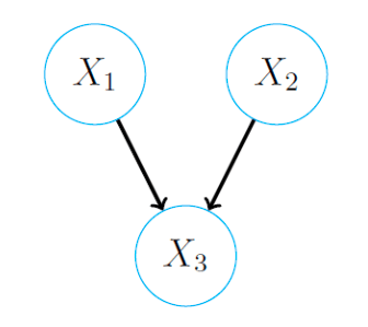
Figure 6: DAG

• All the three variables are binary of values $\{1,2\}$
• We have the following 12 parameters $\theta$
  • For nodes $X_1$, the number configuration of parents is $q_1=1$, which is empty (no parents), so the parameters related to $X_1$$${\theta }_{111}=P(X_1=1)$$$${\theta }_{121}=P(X_1=2)$$

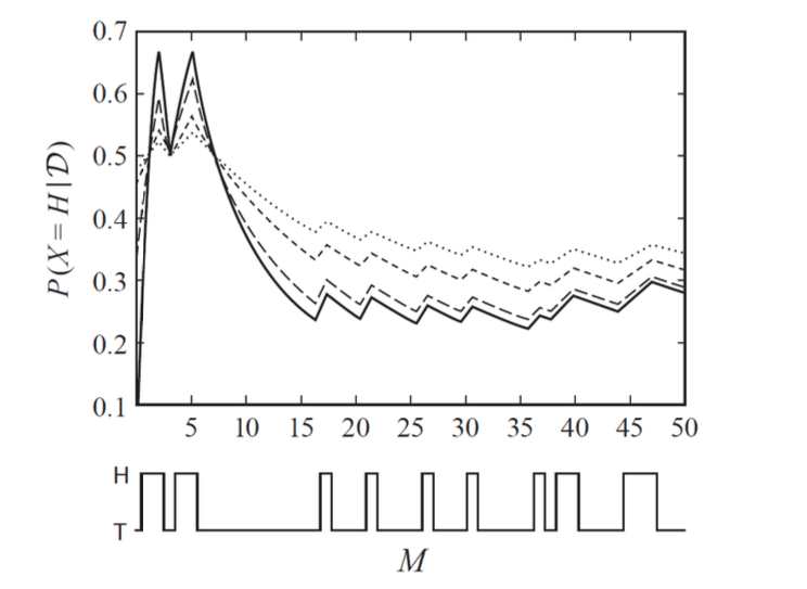
The effect of different priors on smoothing our parameter estimates. The graph shows the estimate of $\theta$ (y-axis) after seeing different number of samples (x-axis). The graph below the x-axis shows the particular sequence of tosses. The solid line corresponds to the MLE estimate, and the remaining ones to Bayesian estimates with different strengths and uniform prior means. The large-dashline corresponds to $Beta(1;1)$, the small-dash line to $Beta(5;5)$, and the dotted line to $Beta(10;10)$.

• It is similar for nodes $X_2$, the number configuration of parents is $q_2=1$, which is also empty, so the parameters related to $X_2$$${\theta }_{211}=P(X_2=1)$$$${\theta }_{221}=P(X_2=2)$$
• For nodes $X_3$, there are 4 different configurations of parents, $q_3=2^2$

  • $P{a}_{X_i}=1:(X_1=1,X_2=1)$

    $${\theta }_{311}=P(X_3=1\mid X_1=1,X_2=1){\theta }_{321}=P(X_3=2\mid X_1=1,X_2=1)$$

  • $P{a}_{X_i}=2:(X_1=1,X_2=2)$

    $${\theta }_{312}=P(X_3=1\mid X_1=1,X_2=2){\theta }_{322}=P(X_3=2\mid X_1=1,X_2=2)$$

  • $P{a}_{X_i}=3:(X_1=2,X_2=1)$

    $${\theta }_{313}=P(X_3=1\mid X_1=2,X_2=1){\theta }_{323}=P(X_3=2\mid X_1=2,X_2=1)$$

  • $P{a}_{X_i}=4:(X_1=2,X_2=2)$

    $${\theta }_{314}=P(X_3=1\mid X_1=2,X_2=2){\theta }_{324}=P(X_3=2\mid X_1=2,X_2=2)$$
• Data
  • Given a complete case $D_l$: a vector of values, one for each variable
  • $D_1=(X_1=1,X_2=2,X_3=2)$
  • Given a set of complete data cases: $D=\{D_1,D_2,\dots ,D_n\}$

Case for Complete Data sets:

$X_1$	$X_2$	$X_3$
1	1	1
1	1	2
1	1	2
1	2	2
1	2	2
1	2	2
2	1	1
2	1	1
2	1	1
2	1	2
2	2	1
2	2	1
2	2	2
2	2	2
2	2	2
2	2	2

• Find the ML estimates of the parameters $\theta$

Log-likelihood function:

$$\ell (\theta ;D)=\log L(\theta ;D)=\log \prod _{l=1}^{n}P(D_l\mid \theta )=\sum _{l=1}^n\log P(D_l\mid \theta )$$

• For each term $\log P(D_l\mid \theta )$ if $D_l=(1,2,2)$, we will need these three parameters: ${\theta }_{111}=P(X_1=1)$, ${\theta }_{221}=P(X_2=2)$, ${\theta }_{322}=P(X_3=2\mid X_1=1,X_2=2)$ for $P{a}_{X_i}=2$.

$$\log P(D_4\mid \theta )=\log P(X_1=1,X_2=2,X_3=2)$$$$=\log [P(X_1=1\mid \theta )P(X_2=2\mid \theta )P(X_3=2\mid X_1=1,X_2=2,\theta )]$$$$=\log {\theta }_{111}+\log {\theta }_{221}+\log {\theta }_{322}$$

• Define the characteristic function to identify the parameters involved with given data $D_l$$$\chi (i,j,k:D_l)=\{\begin{array}{ll}1& X_i=j,P{a}_{X_i}=k\\ 0& \text{otherwise}\end{array}$$

When $l=4$, the 4th data case: $D_4=(1,2,2)$ $$ \chi(i, j, k: D_4) = \chi(2, 2, 1: D_4) = \chi(3, 2, 2: D_4) = 1 $$ $$ \chi(i, j, k: D_4) = 0 $$

• Logarithm:

  $$\log P(D_l\mid \theta )=\sum _{i,j,k}\chi (i,j,k:D_l)\log {\theta }_{ijk}$$

• Define another function of number of data cases where $X_i=j$ and $P{a}_{X_i}=k$

  $$m_{ijk}=\sum _l\chi (i,j,k:D_l)$$

• We have the MLE for ${\theta }_{ijk}$

$${\theta }_{ijk}^{\ast }=\frac{m_{ijk}}{\sum _j{m}_{ijk}}$$

• Results:MLE for
  • $P(X_1=1)=6/16$
  • $P(X_2=1)=7/16$
  • $P(X_3=1\mid X_1=2,X_2=2)=2/6$
  • ...

Example:

$X_1$	$X_2$	$X_3$
1	1	1
1	1	2
1	1	2
1	2	2
1	2	2
1	2	2
2	1	1
2	1	1
2	1	1
2	1	2
2	2	1
2	2	1
2	2	2
2	2	2
2	2	2
2	2	2

• Summary
  • $\theta$ is a random variable
  • Prior $p(\theta )$: Dirichlet distribution
  • Posterior $p(\theta \mid D)$ also produce Dirichlet distribution

Case for Incomplete Data sets

$X_1$	$X_2$	$X_3$
1	1	1
?	1	2
1	?	?
2	1	1
2	1	1
2	1	2
2	?	1
?	2	?

Incomplete data set ? indicates missing values

	$X_1$	$X_2$	$X_3$
$D_1$	1	1	1
$D_2$	2	2	2
$D_3$	1	-	1
$D_4$	2	-	1

	$X_1$	$X_2$	$X_3$
$D_1$	1	1	1
$D_2$	2	2	2
$D_{3,1}$	1	1	1
$D_{3,2}$	1	2	1
$D_{4,1}$	2	1	2
$D_{4,2}$	2	2	2

---

Missing at random (MAR) assumption: actually value of X and the even X-is-missing ($\alpha$) are conditionally independent given other observed variables

$$P(X|\alpha ,E)=P(X|E)$$

given all the observed variables, the fact that X is missing $\alpha$ gives no additional information about the value.

Expectation-maximization (EM) algorithm:

• An iterative algorithm
• start with an initial estimation ${\theta }^0$
  • at each iteration $t$
    • expectation: complete the data based on ${\theta }^t$
    • maximization: using the completed dataset re-estimate the parameter ${\theta }^{t+1}$
  • after data completion, we obtain a dataset with complete data cases
  • EM re-estimates the parameters using the complete data set.

Example: consider an incomplete data case $D_3=(1,?,?)$

1. General Concept: Splitting Incomplete Cases

In the E-step, an incomplete data point is not assigned a single value. Instead, it is split into multiple "partial data cases," each representing a possible completion. The weight of each partial case corresponds to the posterior probability of that specific completion given the observed data and current parameters.

Illustrative Example: Consider a data point $D_3=(1,?,?)$ where both $X_2$ and $X_3$ are missing. With binary variables, there are $2\times 2=4$ possible completions. The EM algorithm splits $D_3$ into 4 partial cases, weighting them by their conditional probabilities:

$$D_3=(1,?,?)\to \{\begin{array}{ll}{w}_1\cdot (1,1,1)& \text{where }{w}_1=P(X_2=1,X_3=1\mid X_1=1,{\theta }^t)\\ w_2\cdot (1,2,1)& \text{where }{w}_2=P(X_2=2,X_3=1\mid X_1=1,{\theta }^t)\\ w_3\cdot (1,1,2)& \text{where }{w}_3=P(X_2=1,X_3=2\mid X_1=1,{\theta }^t)\\ w_4\cdot (1,2,2)& \text{where }{w}_4=P(X_2=2,X_3=2\mid X_1=1,{\theta }^t)\end{array}$$

---

Worked Example: $X_1\to X_2\to X_3$​

Problem Definition: We wish to estimate parameters for the chain $X_1\to X_2\to X_3$ using an incomplete dataset where $X_2$ is missing in some cases.

Dataset:

• $D_1=(1,1,1)$
• $D_2=(2,2,2)$
• $D_3=(1,?,1)$
• $D_4=(2,?,2)$

Step 1: Initialization $({\theta }^0)$

We begin with an initial guess for the parameters ${\theta }^0$.

$X_1$	1	2
$P(X_1)$	1/2	1/2

$X_1\mathrm{\setminus }{X}_2$	1	2
1	2/3	1/3
2	1/3	2/3

$X_2\mathrm{\setminus }{X}_3$	1	2
1	1/3	2/3
2	2/3	1/3

Step 2: Iteration 1 - E-Step (Data Completion) We calculate the weights for the missing values in $D_3$ and $D_4$ using the current parameters ${\theta }^0$.

Case D3​=(1,?,1): We calculate the likelihood of the missing variable $X_2$ being 1 or 2, given observed $X_1=1,X_3=1$.

• Path A ($X_2=1$): $P(1)P(1|1)P(1|1)=\frac{1}{2}\cdot \frac{2}{3}\cdot \frac{2}{3}=\frac{4}{18}$

• Path B ($X_2=2$): $P(1)P(2|1)P(1|2)=\frac{1}{2}\cdot \frac{1}{3}\cdot \frac{1}{3}=\frac{1}{18}$

• Total Probability: $\frac{5}{18}$

• Weights:

  • $w(X_2=1)=\frac{4/18}{5/18}=\frac{\mathbf{4}}{\mathbf{5}}$
  • $w(X_2=2)=\frac{1/18}{5/18}=\frac{\mathbf{1}}{\mathbf{5}}$

Case D4​=(2,?,2): Similarly, given observed $X_1=2,X_3=2$:

• Path A ($X_2=1$): $P(2)P(1|2)P(2|1)=\frac{1}{2}\cdot \frac{1}{3}\cdot \frac{1}{3}=\frac{1}{18}$

• Path B ($X_2=2$): $P(2)P(2|2)P(2|2)=\frac{1}{2}\cdot \frac{2}{3}\cdot \frac{2}{3}=\frac{4}{18}$

• Weights:

  • $w(X_2=1)=\frac{\mathbf{1}}{\mathbf{5}}$
  • $w(X_2=2)=\frac{\mathbf{4}}{\mathbf{5}}$

Resulting Completed Data Table:

Case ID	$X_1$	$X_2$	$X_3$	Weight
$D_1$	1	1	1	1
$D_2$	2	2	2	1
$D_{3,1}$	1	1	1	4/5
$D_{3,2}$	1	2	1	1/5
$D_{4,1}$	2	1	2	1/5
$D_{4,2}$	2	2	2	4/5

Step 3: Iteration 1 - M-Step (Parameter Re-estimation)

We compute the new parameters ${\theta }^1$ using the weighted counts from the completed table.

1. Update $P(X_1)$:

• Count($X_1=1$) $=1(D_1)+4/5(D_{3,1})+1/5(D_{3,2})=2$
• Count($X_1=2$) $=1(D_2)+1/5(D_{4,1})+4/5(D_{4,2})=2$
• Total samples = 4
• ${\theta }_{X_1=1}^1=\frac{2}{4}=\mathbf{0.5}$

2. Update $P(X_2\mid X_1)$:

• For $X_1=1$ (Total weight = 2.0):

  • $X_2=1$: Weight is $1(D_1)+4/5(D_{3,1})=1.8$ $\to$ Prob $=\frac{1.8}{2.0}=\frac{\mathbf{9}}{\mathbf{10}}$
  • $X_2=2$: Weight is $1/5(D_{3,2})=0.2$ $\to$ Prob $=\frac{0.2}{2.0}=\frac{\mathbf{1}}{\mathbf{10}}$

• For $X_1=2$ (Total weight = 2.0):

  • $X_2=1$: Weight is $1/5(D_{4,1})=0.2$ $\to$ Prob $=\frac{0.2}{2.0}=\frac{\mathbf{1}}{\mathbf{10}}$
  • $X_2=2$: Weight is $1(D_2)+4/5(D_{4,2})=1.8$ $\to$ Prob $=\frac{1.8}{2.0}=\frac{\mathbf{9}}{\mathbf{10}}$

Updated Parameters ${\theta }^1$:

$P(X_1)$
$X_1=1$	0.5
$X_1=2$	0.5

$X_1\mathrm{\setminus }{X}_2$	1	2
$X_1=1$	9/10	1/10
$X_1=2$	1/10	9/10

$X_2\mathrm{\setminus }{X}_3$	1	2
$X_2=1$	9/10	1/10
$X_2=2$	1/10	9/10

---

Key takeaway

Simple MLE and MAP for coin and Dice

• MLE $\frac{n_H}{n_H+n_T}$
• Multinomial MLE ${\theta }_i^{\ast }=\frac{n_i}{n}$
• MAP $\frac{n_H+{\alpha }_H}{n+\alpha }$
• Multinomial MAP $P(D_{n+1}=x_i\mid D)=\frac{n_i+{\alpha }_i}{n+\alpha }$

---

Estimate CPD without Missing Value

Estimate CPD by MLE

$$P(X=x\mid Pa(X)=pa)=\frac{\text{计数}(X=x\cap Pa(X)=pa)}{\text{计数}(Pa(X)=pa)}$$

• 每个节点的 CPD 独立计算 (得益于网络的局部分解)。
• 只需一次遍历数据集进行计数统计。
• 若某父节点配置未出现（计数=0），概率为 0，可用 Laplace 平滑避免：加 1（或伪计数 $\alpha$）到分子分母。

优点:

• 简单、 高效、大样本时准确。

缺点:

• 小样本易过拟合，
• 不确定性度量，
• 无先验。

Estimate CPD by Bayesian Estimation

$${\hat{\theta }}_{ijk}=\frac{m_{ijk}+{\alpha }_{ijk}}{\sum _j{m}_{i{j}^{\prime }k}+\sum _j{\alpha }_{i{j}^{\prime }k}}$$

• $m_{ijk}$ 是 MLE 中的真实计数。
• ${\alpha }_{ijk}$ 是先验提供的伪计数（pseudo-counts）。

Estimate CPD with Missing Value

EM算法的原理

• EM是一种迭代优化算法，旨在最大化不完整数据的对数似然函数。
• 假设缺失值为MAR（Missing At Random），即缺失机制只依赖于观测到的变量。

EM算法步骤（基于完整数据MLE的迭代）

1. 初始化
   选取初始参数 $\theta$（可以随机初始化、使用完整部分数据估计，或设为均匀分布）。
2. E步（Expectation，期望步）
   使用当前参数 $\theta$ 计算每个缺失值的条件期望概率。
   • 将不完整实例“软分割”成多个完整实例（每个配置的权重为其条件概率）。
   • 由此得到一个加权的“完整”数据集。
3. M步（Maximization，最大化步）
   在加权的完整数据集上执行加权MLE（使用加权频率计数），得到新的参数 $\theta$。
   • 本质上是将参数估计公式中的计数替换为加权计数。

Example

本案例演示从完整数据中估计条件概率分布（CPD）的过程。

假设三个二值变量 X1、X2、X3（取值 0 或 1），贝叶斯网络结构为 X1 → X2 → X3。

联合概率分解为：

$$P(X_1,X_2,X_3)=P(X_1)\times P(X_2|X_1)\times P(X_3|X_1,X_2)$$

数据集

有 4 个完整观测实例：

实例	X1	X2	X3
D1	1	1	1
D2	1	0	1
D3	0	1	0
D4	0	0	0

参数估计（最大似然估计 MLE）

1. P(X1)
   $P(X1=1)=\frac{2}{4}=0.5$$P(X1=0)=0.5$

2. P(X2 | X1)

   • 当 $X_1=1$ 时：计数 $X_2=1$ 有 1 个（D1），总计 2 个 → $P(X2=1|X1=1)=\frac{1}{2}=0.5$
     $P(X2=0|X1=1)=0.5$
   • 当 X1=0 时：计数 X2=1 有 1 个（D3），总计 2 个 → $P(X2=1|X1=0)=0.5$
     $P(X2=0|X1=0)=0.5$

3. P(X3 | X1, X2)

   • $(X1=1,X2=1)：\mathrm{仅}D1，X3=1\to P(X3=1|X1=1,X2=1)=1.0$
   • $(X1=1,X2=0)：\mathrm{仅}D2，X3=1\to P(X3=1|X1=1,X2=0)=1.0$
   • $(X1=0,X2=1)：\mathrm{仅}D3，X3=0\to P(X3=1|X1=0,X2=1)=0.0$
   • $(X1=0,X2=0)：\mathrm{仅}D4，X3=0\to P(X3=1|X1=0,X2=0)=0.0$