Numerical Computation Fundamentals

Binary numbers

Binary numbers are expressed as

$$...b_2{b}_1{b}_0.b_{-1}{b}_{-2}...$$

where each binary digit, or bit, is 0 or 1. The base 10 equivalent to the number is

$$...b_2{2}^2+b_1{2}^1+b_0{2}^0+b_{-1}{2}^{-1}+b_{-2}{2}^{-2}...$$

EXAMPLE:
The decimal number 4 is expressed as $(100.{)}_2$ in base 2, and $3/4$ is represented as $(0.11{)}_2$.

Decimal to Binary

To convert a decimal number to binary, it is simplest to break the number into integer and fractional parts and convert each part separately.

Integer part. Convert decimal integers to binary dividing by 2 successively and recording the remainders.

53 ÷ 2 = 26 R 1
26 ÷ 2 = 13 R 0
13 ÷ 2 = 6  R 1
6  ÷ 2 = 3  R 0
3  ÷ 2 = 1  R 1
1  ÷ 2 = 0  R 1

Therefore, the base 10 number 53 can be written in bits as 110101, denoted as ${53}_{10}={110101}_2$.

Fractional part. Convert $(0.7{)}_{10}$ to binary by reversing the preceding steps. Multiply by 2 successively and record the integer parts, moving away from the decimal point to the right.

0.7 × 2 = 1.4 → 1
0.4 × 2 = 0.8 → 0
0.8 × 2 = 1.6 → 1
0.6 × 2 = 1.2 → 1
0.2 × 2 = 0.4 → 0
0.4 × 2 = 0.8 → 0
...

Therefore, $(0.7{)}_{10}=(.1011001100110\dots {)}_2=(.1\overline{0110}{)}_2$

where overbar notation is used to denote infinitely repeated bits. Putting the two parts together, we conclude that $(53.7{)}_{10}=(110101.1\overline{0110}{)}_2.$

Binary to Decimal

To convert a binary number to decimal, it is again best to separate into integer and fractional parts.

Integer part: Simply add up powers of 2. The binary number $(10101{)}_2$ is simply

$$1\cdot 2^4+0\cdot 2^3+1\cdot 2^2+0\cdot 2^1+1\cdot 2^0=(21{)}_{10}.$$

Fractional part: If the fractional part is finite, proceed the same way

$$(.1011{)}_2=\frac{1}{2}+\frac{1}{8}+\frac{1}{16}={\left(\frac{11}{16}\right)}_{10}.$$

When the fractional part is not a finite base 2 expansion.

EXAMPLE:

When the fractional part is not a finite base 2 expansion, we can use the shift property of multiplication by 2.

Suppose $x=(0.\overline{1011}{)}_2$,

$$2^{4}x=1011.\overline{1011}$$$$x=0000.\overline{1011}$$

Subtracting yields

$$(2^4-1)x=(1011{)}_2=(11{)}_{10}$$

Then solve for $x$ to find

$$x=(0.\overline{1011}{)}_2={\left(\frac{11}{15}\right)}_{10}.$$

Floating point representation of real numbers

A floating point number consists of three parts: the sign (+ or −), a mantissa, which contains the string of significant bits, and an exponent. The three parts are stored together in a single computer word. The form of a normalized floating point number is

$$\pm 1.bbb\dots b\times 2^p$$

where each of the $N$ $b$'s is 0 or 1, and $p$ is an $M$-bit binary number representing the exponent. Normalization means that the leading bit must be 1.

The double precision format, common in C compilers, Python, and MATLAB, uses exponent length $M=11$ and mantissa length $N=52$.

The floating-point form of $y$ is obtained by terminating the mantissa of $y$ at $k$ decimal digits.

Chopping

Chop off the digits $d_{k+1}{d}_{k+2}\dots$

$$fl(y)=0.d_1{d}_2\dots d_k\times {10}^n$$

Rounding

Adds $5\times {10}^{n-(k+1)}$ to $y$ and then chops the result to obtain a number of the form

$$fl(y)=0.{\delta }_1{\delta }_2\dots {\delta }_k\times {10}^n$$

When $d_{k+1}\ge 5$, we add $1$ to $d_k$; when $d_{k+1}<5$, we simply chop off all but the first $k$ digits.

EXAMPLE:

(a) The floating-point form of $\pi$ using five-digit chopping is

$$fl(\pi )=0.31415\times {10}^1=3.1415$$

(b) The floating-point form of $\pi$ using five-digit rounding is

$$fl(\pi )=0.31416\times {10}^1=3.1416$$

Correct within 𝑝 decimal places

A Solution is correct within $p$ decimal places if the error is less than $0.5\times {10}^{-p}$

Absolute Error & Relative Error

DEFINITION: Let $x_c$ be a computed version of the exact quantity $x$. Then

$$\mathbf{\text{absolute error}}=|x_c-x|,$$

and

$$\mathbf{\text{relative error}}=\frac{|x_c-x|}{|x|}$$

EXAMPLE:

(a) $x_c=0.3100\times {10}^1,x=0.3000\times {10}^1$

$$\mathbf{\text{absolute error}}=|x_c-x|=|0.3100\times {10}^1-0.3000\times {10}^1|=0.1$$$$\mathbf{\text{relative error}}=\frac{|x_c-x|}{|x|}=\frac{0.1}{|0.3000\times {10}^1|}=0.333\bar{3}\times {10}^{-1}$$

(b) $x_c=0.3100\times {10}^4,x=0.3000\times {10}^4$

$$\mathbf{\text{absolute error}}=|x_c-x|=|0.3100\times {10}^4-0.3000\times {10}^4|=0.1\times {10}^3$$$$\mathbf{\text{relative error}}=\frac{|x_c-x|}{|x|}=\frac{0.1\times {10}^3}{|0.3000\times {10}^4|}=0.333\bar{3}\times {10}^{-1}$$

Same relative error, $0.333\bar{3}\times {10}^{-1}$, occurs for widely varying absolute errors. As a measure of accuracy, the absolute error can be misleading and the relative error more meaningful because the relative error takes into consideration the size of the value.

Loss of significance

Assume that through considerable effort, as part of a long calculation, we have determined two numbers correct to seven significant digits, and now need to subtract them:

$$123.4567-123.4566=000.0001$$

Let’s write the subtraction in normalized decimal float-point:

$$0.1234567\times {10}^3-0.1234566\times {10}^3=0.1\times {10}^{-3}$$

The subtraction problem began with two input numbers that we knew to seven-digit accuracy, and ended with a result that has only one-digit accuracy. It is called loss of significance, and in many cases this can be avoided by restructuring the calculation.

Convergence

To calculate convergence, we usually try to estimate the error in the numerical solution compared to the actual solution. We try to find out how fast this error is decreasing (or increasing).

DEFINITION:

Suppose $\{{\beta }_n{\}}_{n=1}^{\mathrm{\infty }}$ is a sequence converging to zero, and $\{a_n{\}}_{n=1}^{\mathrm{\infty }}$ converges to a number $\alpha$. If a positive constant $K$ exists with

$$|a_n-\alpha |\le K|{\beta }_n|,\text{for large }n,$$

then we say that $\{a_n{\}}_{n=1}^{\mathrm{\infty }}$ converges to $\alpha$ with rate of convergence $O({\beta }_n)$, indicated by $a_n=\alpha +O({\beta }_n)$.

---

DEFINITION:
Let ${\epsilon }_n$ be the error in the $n$th iteration of the algorithm. That is, ${\epsilon }_n=|a_n-\alpha |$.

DEFINITION:
We say that the algorithm has linear convergence if $|{\epsilon }_{n+1}|=C|{\epsilon }_n|$.

DEFINITION:
We say that the algorithm has quadratic convergence if $|{\epsilon }_{n+1}|=C|{\epsilon }_n{|}^2$.

---

设误差为

$$e_i=|x_i-r|$$

其中 $r$ 为方程 $f(x)=0$ 的真根，$x_i$ 为第 $i$ 次迭代的近似值。

若存在常数 $p>0$、$C>0$，使得

$$\underset{i\to \mathrm{\infty }}{lim}\frac{|e_{i+1}|}{|e_i{|}^p}=C<\mathrm{\infty },$$

则称该方法具有 p 阶收敛（order of convergence = p）。

收敛类型	条件	特征	示例
线性收敛（Linear）	$p=1,0<C<1$	误差按比例缩小	二分法、FPI
超线性收敛（Superlinear）	$1<p<2$	介于线性与二次之间	割线法
二次收敛（Quadratic）	$p=2$	误差平方级减少	牛顿法

---

Review of calculus

Limits and Continuity

DEFINITION:

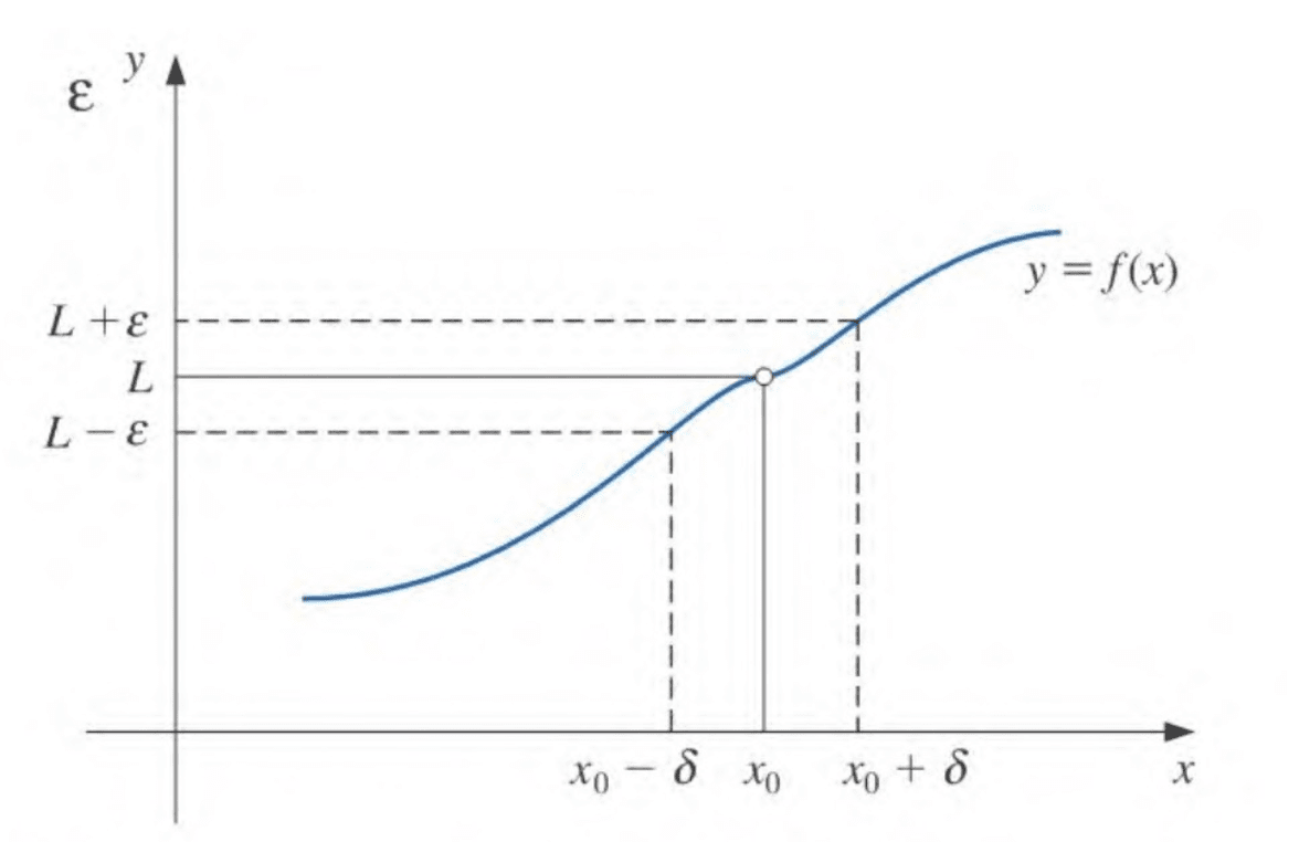
A function $f$ defined on a set $X$ of real numbers has the limit $L$ at $x_0$, written

$$\underset{x\to x_0}{lim}f(x)=L,$$

if, given any real number $\epsilon >0$, there exists a real number $\delta >0$ such that

$$|f(x)-L|<\epsilon$$

whenever $x\in X$ and

$$0<|x-x_0|<\delta .$$

---

DEFINITION:
Let $f$ be a function defined on a set $X$ of real numbers and $x_0\in X$. Then $f$ is continuous at $x_0$ if

$$\underset{x\to x_0}{lim}f(x)=f(x_0).$$

The function $f$ is continuous on the set $X$ if it is continuous at each number in $X$.

DEFINITION:
Let $\{x_n{\}}_{n=1}^{\mathrm{\infty }}$ be an infinite sequence of real numbers. This sequence has the limit $x$ (converges to $x$) if, for any $\epsilon >0$, there exists a positive integer $N(\epsilon )$ such that $|x_n-x|<\epsilon$ whenever $n>N(\epsilon )$. The notation

$$\underset{n\to \mathrm{\infty }}{lim}{x}_n=x,\text{or}{x}_n\to x\text{ as }n\to \mathrm{\infty },$$

means that the sequence $\{x_n{\}}_{n=1}^{\mathrm{\infty }}$ converges to $x$.

THEOREM:
If $f$ is a function defined on a set $X$ of real numbers and $x_0\in X$, then the following statements are equivalent:

a. $f$ is continuous at $x_0$;

b. If $\{x_n{\}}_{n=1}^{\mathrm{\infty }}$ is any sequence in $X$ converging to $x_0$, then

$$\underset{n\to \mathrm{\infty }}{lim}f(x_n)=f(x_0).$$

Differentiability

DEFINITION:
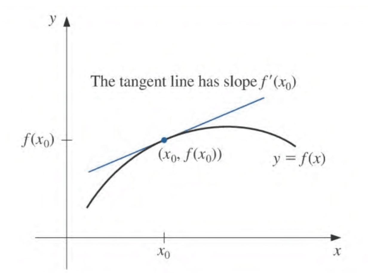
Let $f$ be a function defined on an open interval containing $x_0$. The function $f$ is differentiable at $x_0$ if

$$f^{\prime }(x_0)=\underset{x\to x_0}{lim}\frac{f(x)-f(x_0)}{x-x_0}$$

exists. The number $f^{\prime }(x_0)$ is called the derivative of $f$ at $x_0$. The function that has a derivative at each number in a set $X$ is differentiable on $X$.

THEOREM:
If the function $f$ is differentiable at $x_0$, then $f$ is continuous at $x_0$.

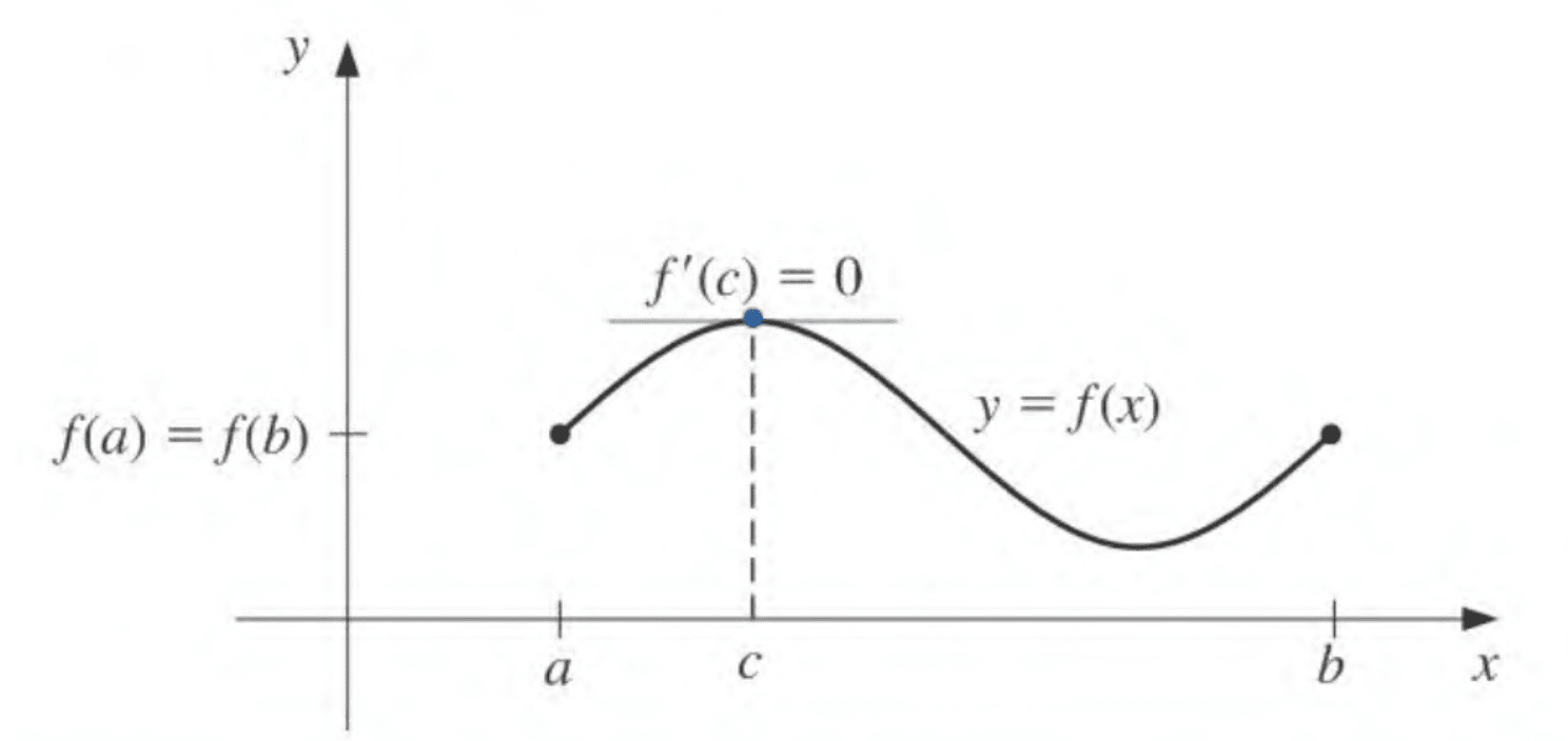
THEOREM (Rolle’s Theorem):
Suppose $f\in C[a,b]$ and $f$ is differentiable on $(a,b)$. If $f(a)=f(b)$, then a number $c$ in $(a,b)$ exists with

$$f^{\prime }(c)=0.$$

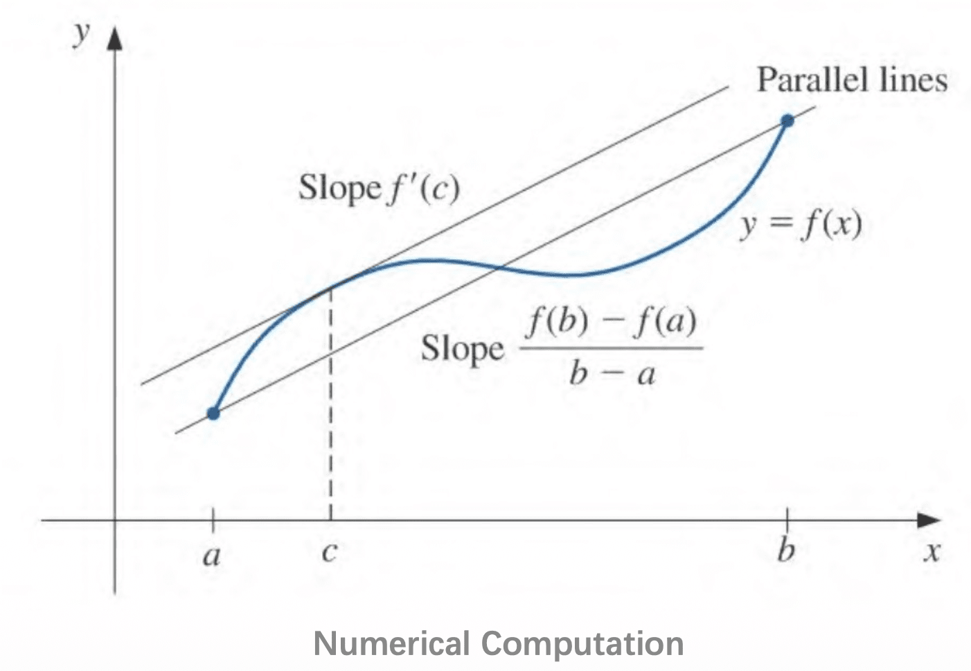
THEOREM (Mean Value Theorem):
If $f\in C[a,b]$ and $f$ is differentiable on $(a,b)$. Then a number $c$ in $(a,b)$ exists with

$$f^{\prime }(c)=\frac{f(b)-f(a)}{b-a}.$$

THEOREM (Intermediate Value Theorem):
If $f\in C[a,b]$ and $K$ is any number between $f(a)$ and $f(b)$, then there exists a number $c$ in $(a,b)$ for which

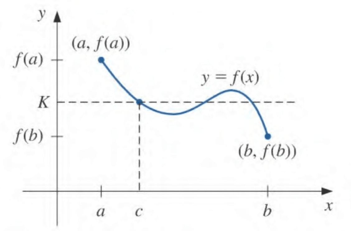
$$f(c)=K.$$

Integration

DEFINITION:
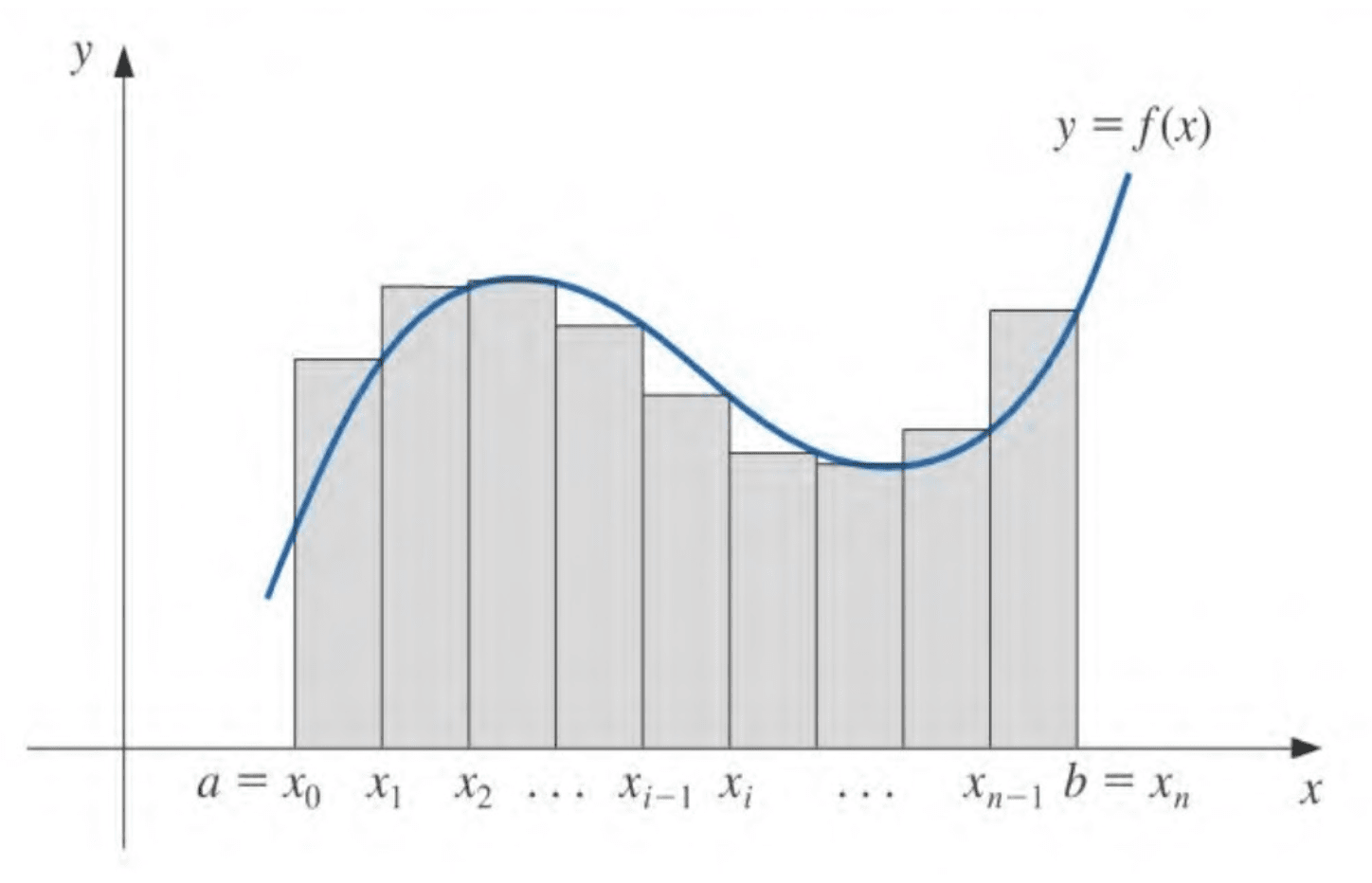
The Riemann integral of the function $f$ on the interval $[a,b]$ is the following limit, provided it exists:

$${\int }_a^{b}f(x)dx=\underset{\mathrm{\Delta }{x}_i\to 0}{lim}\sum _{i=1}^{n}f(z_i)\mathrm{\Delta }{x}_i,$$

where the numbers $x_0,x_1,...,x_n$ satisfy $a=x_0\le x_1\le ...\le x_n=b$, where $\mathrm{\Delta }{x}_i=x_i-x_{i-1}$, for each $i=1,2,...,n$, and $z_i$ is arbitrarily chosen in the interval $[x_{i-1},x_i]$.

Taylor Polynomials and Series

THEOREM (Taylor’s Theorem):
Suppose $f\in C^n[a,b]$, $f^{(n+1)}$ exists on $[a,b]$, and $x_0\in [a,b]$. For every $x\in [a,b]$, there exists a number $\xi (x)$ between $x_0$ and $x$ with

$$f(x)=P_n(x)+R_n(x),$$

where

$$P_n(x)=f(x_0)+f^{\prime }(x_0)(x-x_0)+\frac{f^{″}(x_0)}{2!}(x-x_0{)}^2+\cdots +\frac{f^{(n)}(x_0)}{n!}(x-x_0{)}^n=\sum _{k=0}^n\frac{f^{(k)}(x_0)}{k!}(x-x_0{)}^k$$

and

$$R_n(x)=\frac{f^{(n+1)}(\xi (x))}{(n+1)!}(x-x_0{)}^{n+1}.$$

Here $P_n(x)$ is called the nth Taylor polynomial for $f$ about $x_0$, and $R_n(x)$ is called the remainder term (or truncation error) associated with $P_n(x)$.

The infinite series obtained by taking the limit of $P_n(x)$ as $n\to \mathrm{\infty }$ is called the Taylor series for $f$ about $x_0$. In the case $x_0=0$, the Taylor polynomial is often called a Maclaurin polynomial, and the Taylor series is often called a Maclaurin series.

The term truncation error in the Taylor polynomial refers to the error involved in using a truncated, or finite, summation to approximate the sum of an infinite series.

Example

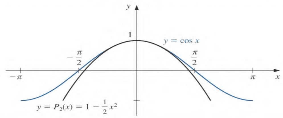
Let $f(x)=\cos x$ and $x_0=0$. Determine
a. The second Taylor polynomial for $f$ about $x_0$; and
b. The third Taylor polynomial for $f$ about $x_0$.

---

SOLUTION:

$$f^{\prime }(x)=-\sin x,f^{″}(x)=-\cos x,f^{‴}(x)=\sin x,\text{and }{f}^{(4)}(x)=\cos x,$$

So

$$f(0)=1,f^{\prime }(0)=0,f^{″}(0)=-1,\text{and }{f}^{‴}(0)=0.$$

a.

$$\cos x=f(0)+f^{\prime }(0)x+\frac{f^{″}(0)}{2!}{x}^2+\frac{f^{‴}(\xi (x))}{3!}{x}^3$$

where $\xi (x)$ is some number between 0 and $x$.

$$\cos x=1-\frac{1}{2}{x}^2+\frac{1}{6}{x}^3\sin \xi (x),$$

When $x=0.01$, this becomes

$$\cos 0.01=1-\frac{1}{2}(0.01{)}^2+\frac{1}{6}(0.01{)}^3\sin \xi (0.01),$$$$=0.99995+\frac{{10}^{-6}}{6}\sin \xi (0.01).$$

Since $-1\le \sin \xi (0.01)\le 1$,

$$0.99994998<0.99995-1.6\times {10}^{-7}\le \cos 0.01\le 0.99995+1.6\times {10}^{-7}<0.9999502.$$

Furthermore, since $|\sin x|\le |x|$, we have

$$-0.01\le \sin \xi (0.01)\le 0.01.$$

Substitute into the remainder, the error is in the region

$$[-1.6\times {10}^{-9},1.6\times {10}^{-9}].$$

b. Since $f^{‴}(0)=0$, the third Taylor polynomial with remainder term about $x_0=0$ is

$$\cos x=1-\frac{1}{2}{x}^2+\frac{1}{24}{x}^4\cos \xi (x),$$

where $0<\xi (x)<0.01$.

The approximating polynomial remains the same, and the approximation is still $0.99995$, but we now have much better accuracy assurance. Since $-1\le \cos \xi (x)\le 1$ for all $x$, we have

$$|\frac{1}{24}{x}^4\cos \xi (x)|\le \frac{1}{24}(0.01{)}^4(1)\approx 4.2\times {10}^{-10}.$$

So,

$$0.99994999958<0.99995-4.2\times {10}^{-10}\le \cos 0.01\le 0.99995+4.2\times {10}^{-10}<0.99995000042.$$